The Art of Unpredictability
Why Randomness is Rational

The Game That Refused to Settle

In Chapter Three, we introduced Nash equilibrium and found it in several games — Prisoner's Dilemma, Stag Hunt, Battle of the Sexes. In each case, we could identify at least one pair of pure strategies where neither player had an incentive to deviate. But we also encountered a game that refused to cooperate with our analysis: Matching Pennies.

Recall the setup. Two players simultaneously choose Heads or Tails. Player One, the Matcher, wins if the coins match; Player Two, the Mismatcher, wins if they differ. In the payoff matrix, Player One's payoff is listed first. If both choose Heads or both choose Tails, Player One gets plus one and Player Two gets minus one. If choices differ, Player One gets minus one and Player Two gets plus one.

We checked every cell. If Player One plays Heads, Player Two wants to play Tails. But if Player Two plays Tails, Player One also wants to play Tails. Then Player Two wants to switch to Heads, and so the cycle continues. No pair of pure strategies is stable — there is no pure-strategy Nash equilibrium.

This is not a quirky edge case. Many real strategic situations share this cycling structure: a goalkeeper facing a penalty kicker, a tennis player choosing where to serve, a military commander deciding which route to patrol, a poker player deciding whether to bluff. In each case, predictability is death. If your opponent knows what you will do, they can exploit you. The question is: what should a rational player do when every deterministic choice can be punished?

Mixed Strategies · A Probability Distribution Over Choices

The answer to our puzzle requires expanding what we mean by a "strategy." So far, a strategy has meant a definite choice: play Heads, or play Tails. We call these pure strategies — complete specifications of what to do with certainty. A mixed strategy is something different: it is a probability distribution over pure strategies. Instead of choosing Heads or Tails, you choose Heads with probability p and Tails with probability one minus p.

This is not the same as being indecisive or confused. A mixed strategy is a deliberate, calculated plan. Think of it as programming a random device — perhaps rolling a die, or checking the second hand on your watch — and committing in advance to follow whatever it dictates. The crucial feature is that even you do not know exactly what you will do in any given instance. And if you do not know, your opponent certainly cannot know.

Expected Utility

If strategies now involve probabilities, we need a way to evaluate them. Enter expected utility — the probability-weighted average of the payoffs from each possible outcome. This concept, formalised by von Neumann and Morgenstern in nineteen forty-four in their foundational treatise, allows us to compare random prospects on a common scale.

Suppose Player One plays Heads with probability p and Tails with probability one minus p, while Player Two plays Heads with probability q and Tails with probability one minus q. Since the players choose independently, the probability of any outcome is the product of the individual probabilities. The expected utility for Player One is: p times q times plus one, plus p times one minus q times minus one, plus one minus p times q times minus one, plus one minus p times one minus q times plus one.

Expanding and simplifying, the expected utility for Player One equals four pq minus two p minus two q plus one. This is the function Player One wants to maximise by choosing p, knowing that Player Two is choosing q to minimise it, since this is a zero-sum game. But how do we find the right values of p and q?

The Indifference Principle

Here is the key insight, and it is worth pausing to appreciate just how elegant it is. In a mixed-strategy Nash equilibrium, each player's mixture must make the other player indifferent between their pure strategies. This is the indifference principle, and it is the engine that drives every mixed-strategy calculation you will ever do, as Osborne and Rubinstein described in nineteen ninety-four.

Why must this be true? Think about it from Player Two's perspective. Player Two is mixing between Heads and Tails. But Player Two would only be willing to randomise if both options give the same expected payoff. If Heads gave a higher expected payoff than Tails, Player Two would play Heads with certainty — and we would be back to a pure strategy. For Player Two to genuinely randomise, she must be indifferent. And what determines Player Two's expected payoff from each option? Player One's mixture. So Player One's mixing probability is determined by the requirement that Player Two is indifferent.

This produces a beautiful and slightly paradoxical result: each player's equilibrium mixture is chosen not to optimise their own payoff directly, but to make their opponent unable to exploit them. Your mixture is your opponent's problem to solve, and their mixture is yours.

Solving Matching Pennies

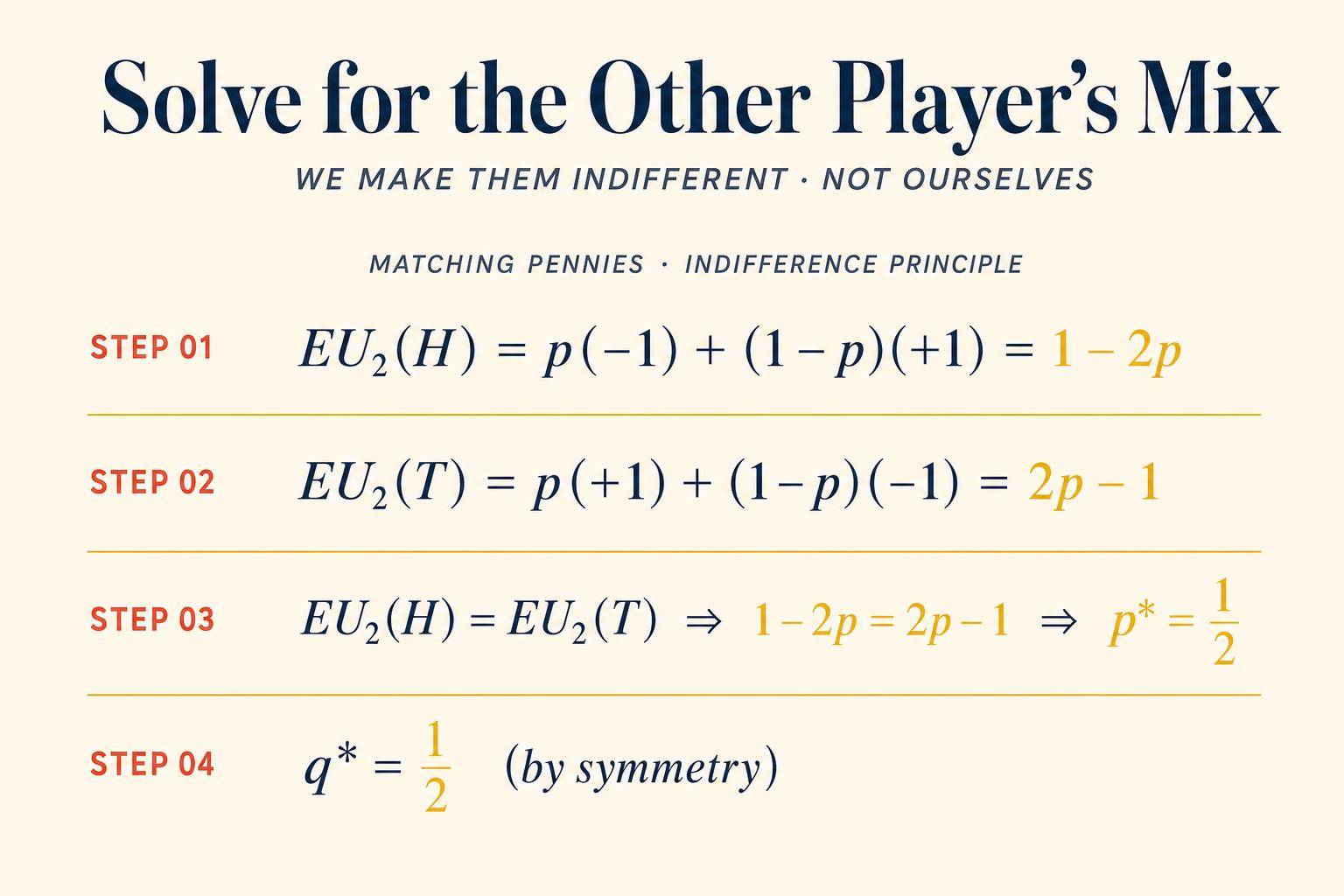
Let's apply the indifference principle to Matching Pennies. Player One plays Heads with probability p. We need to find the value of p that makes Player Two indifferent.

Player Two's expected payoff from playing Heads: With probability p, Player One also plays Heads and Player Two gets minus one. With probability one minus p, Player One plays Tails and Player Two gets plus one. So the expected utility for Player Two from playing Heads equals p times minus one plus one minus p times plus one, which simplifies to one minus two p.

Player Two's expected payoff from playing Tails equals p times plus one plus one minus p times minus one, which simplifies to two p minus one.

Setting them equal: one minus two p equals two p minus one, which gives four p equals two, so p equals one half.

By the same logic — the game is symmetric — Player Two must play Heads with probability q equals one half. The mixed-strategy Nash equilibrium is for both players to randomise fifty-fifty — exactly the intuitive answer. Each player's expected payoff at equilibrium is zero, which makes sense: in a fair, symmetric zero-sum game, neither side can expect to gain an advantage.

Asymmetric Games · Attacker-Defender

Matching Pennies is symmetric, so the equilibrium is an even split. Most real games are not symmetric. Consider a modified game — let's call it Attacker-Defender — with the following payoffs for the Row player. If Row plays A and Column plays A, Row gets two and Column gets minus two. If Row plays A and Column plays B, Row gets minus one and Column gets one. If Row plays B and Column plays A, Row gets minus one and Column gets one. If Row plays B and Column plays B, Row gets three and Column gets minus three.

Let Row play A with probability p. Column's expected payoff from playing A equals p times minus two plus one minus p times one, which is one minus three p. Column's expected payoff from playing B equals p times one plus one minus p times minus three, which is four p minus three. Setting equal: one minus three p equals four p minus three, so seven p equals four, giving p equals four sevenths, approximately zero point five seven one.

Notice what happened: because Row's payoff from B when Column plays B is higher than from A when Column plays A, Row plays A more often, not less. This is not to favour A directly — it is to keep Column guessing. The asymmetry in payoffs generates asymmetry in the equilibrium mixture.

Penalty Kicks · The Theory Meets the Pitch

Mixed-strategy Nash equilibrium is a beautiful theoretical construct. But does anyone actually play this way? The theory demands that players randomise with precise probabilities and generate statistically independent sequences — no patterns, no streaks, no predictability. That's a tall order for flesh-and-blood humans. Many laboratory experiments have found that undergraduate subjects deviate substantially from equilibrium predictions. So is mixed-strategy equilibrium just an elegant fiction?

Enter the penalty kick.

Ignacio Palacios-Huerta had a brilliant idea: instead of testing game theory in artificial lab settings, look at professional athletes who face the same strategic problem repeatedly, with enormous stakes, and years of experience. A penalty kick is, in essence, a simultaneous-move, zero-sum game. The kicker chooses a side; the goalkeeper chooses a side to dive. The ball travels too fast for reactive adjustment. The payoffs are asymmetric — kickers are typically stronger on their "natural" side, right foot shooting to the left for right-footed kickers, and goalkeepers know this.

As Palacios-Huerta reported in two thousand three, he analysed one thousand four hundred seventeen penalty kicks from top European leagues between nineteen ninety-five and two thousand. The mixed-strategy Nash equilibrium for this game makes two precise predictions. First, equal scoring rates: The probability of scoring should be the same regardless of which direction the kicker chooses. If scoring were more likely on one side, a rational kicker would shift more kicks there, which would cause the goalkeeper to shift as well, until scoring rates equalised. Second, serial independence: Each kick should be statistically independent of previous kicks. No patterns, no alternation bias, no streaks — pure randomness.

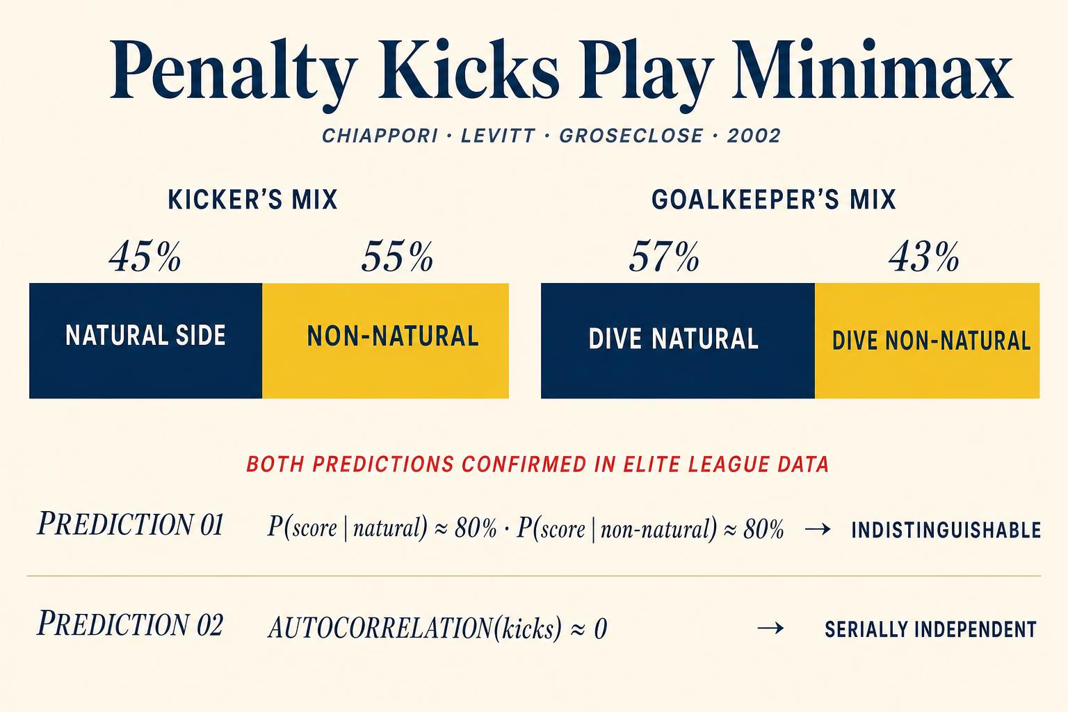
The results were striking. Scoring rates were approximately eighty percent regardless of the direction chosen — statistically indistinguishable across strategies, exactly as the theory predicts. The sequences showed no significant serial correlation: knowing a kicker's previous choices gave no useful information about the next one. Professional footballers, shaped by years of competitive pressure and implicit learning, had converged on behaviour virtually indistinguishable from the mixed-strategy Nash equilibrium.

As Chiappori, Levitt, and Groseclose reported in two thousand two, they reached similar conclusions using a different dataset of four hundred fifty-nine kicks, while also developing methods to account for heterogeneity across individual kickers and goalkeepers. They found that kickers went to their natural side about forty-five percent of the time, while goalkeepers dove to the kicker's natural side about fifty-seven percent of the time — exactly the pattern predicted by equilibrium given the asymmetric payoffs. Azar and Bar-Eli extended these tests in two thousand eleven to additional leagues and tournaments, confirming that the mixed-strategy Nash equilibrium consistently outperforms alternative prediction methods.

Walker and Wooders found similar patterns in two thousand one in professional tennis serves at Wimbledon: servers varied the direction of their serves in ways that approximately equalised their success rates across locations, as the theory predicts. There was some evidence of slight serial correlation — players alternated a bit too much — but the overall picture was remarkably consistent with minimax play.

When the stakes are high, the feedback is clear, and players have extensive experience, mixed-strategy equilibrium is not just a theoretical ideal — it is an accurate description of how experts actually behave.

Palacios-Huerta · Chiappori, Levitt & Groseclose · Walker & Wooders

Unpredictability in War · Security · Deterrence

If penalty kicks provide the most elegant test of mixed-strategy theory, military strategy provides the most consequential application. The logic is identical: a defender who patrols the same route at the same time every day will be ambushed. A bomber that always attacks from the same direction will be shot down. Predictability in conflict is not just suboptimal — it is lethal.

During World War Two, British Operational Research teams grappled with exactly this problem. As Rau documented in two thousand five, scientists embedded with the military applied quantitative methods to problems ranging from convoy routing to anti-submarine patrol patterns. A key insight was that patrol routes needed to be randomised. If German U-boats could predict where Allied patrols would search, they could simply avoid those areas. By randomising patrol routes — while maintaining coverage probabilities that matched the threat level in each zone — Allied forces could maximise the probability of detection without becoming predictable.

The same logic extended to strategic deception. Before D-Day, the Allies went to extraordinary lengths to make the location of the invasion unpredictable. Operation Fortitude created an entirely fictitious army group, complete with inflatable tanks and fake radio traffic, to convince the Germans that the invasion would target Pas-de-Calais rather than Normandy. The strategic logic was fundamentally about mixed strategies: even after the Normandy landings began, the Germans hesitated to commit their reserves, believing the "real" invasion might still come at Calais. By maintaining uncertainty about their intentions, the Allies forced the Germans into a defensive posture that was spread too thin.

In the nuclear age, unpredictability became even more central to strategic thinking. The doctrine of nuclear deterrence rested partly on maintaining ambiguity about the precise conditions that would trigger a nuclear response. As Thomas Schelling argued — whose work on commitment we will encounter in Chapter Six — if an adversary knew the exact "red line," they could engage in provocations that fell just short of it. A degree of calculated unpredictability — what Schelling called "the threat that leaves something to chance" — could actually be stabilising, because it prevented adversaries from fine-tuning their provocations.

The Minimax Theorem · von Neumann's Guarantee

We have now seen that mixed strategies can solve the problem of games like Matching Pennies that have no pure-strategy equilibrium. But how general is this? Could there be some other game — perhaps with three or four strategies per player — where even mixing fails to produce an equilibrium?

The answer is no, and the reason is one of the most important results in all of game theory: the minimax theorem, proved by John von Neumann in nineteen twenty-eight. For any finite two-person zero-sum game, von Neumann showed that the maximum payoff that Player One can guarantee by choosing the best mixture assuming Player Two will respond optimally equals the minimum payoff that Player Two can force upon Player One by choosing the best countermixture. This common value is the value of the game, and the strategies that achieve it constitute the equilibrium.

Why is this so important? Because without mixing, the maximin and minimax values can differ. In Matching Pennies with pure strategies, Player One's maximin value is minus one — the best guarantee is to play either side and lose whenever the opponent guesses right — while the minimax value is plus one. There's a gap. Mixing closes this gap. By randomising fifty-fifty, Player One guarantees an expected payoff of zero regardless of what Player Two does. And Player Two cannot force a lower expected payoff than zero regardless of what Player One does. The gap vanishes.

Von Neumann and Morgenstern extended this foundation considerably in nineteen forty-four, developing the expected utility theory that makes the entire framework rigorous. Their utility axioms — showing that under reasonable assumptions about preferences, individuals behave as if they maximise expected utility — gave mixed strategies a solid decision-theoretic foundation. John Nash would later extend the existence result beyond zero-sum games to all finite games, a topic for Chapter Five, but von Neumann's minimax theorem was the crucial first step.

The minimax theorem tells us that the equilibrium mixture is special: it is the unique probability that maximises your worst-case expected payoff. Deviate from it in either direction, and an omniscient opponent can punish you more severely.

Three Interpretations of "Randomisation"

Mixed strategies raise a deep interpretive question: do real players actually randomise? Do they literally flip mental coins before making decisions? The answer is nuanced, and it is worth being honest about the different interpretations that game theorists offer.

The most literal interpretation is that players deliberately introduce randomness into their decision-making. A poker player might use the second hand of their watch to determine whether to bluff: if it's an even number, bluff; odd, don't. This interpretation is most plausible in repeated competitive settings — like penalty kicks or poker — where the cost of being predictable is immediate and obvious.

An alternative view is that mixed-strategy equilibrium describes the population frequencies rather than any individual's randomisation. In a large population of players, some always play Heads and some always play Tails. The equilibrium mixture, fifty-fifty in Matching Pennies, describes the fraction of the population choosing each strategy. Each individual plays a pure strategy, but the aggregate looks random.

A third interpretation, common in modern game theory, is that a player's mixed strategy represents the opponent's beliefs about what the player will do. Player Two's belief that Player One plays Heads with probability one half could arise because Player One actually randomises, or because Player Two is uncertain about Player One's "type" or decision procedure. Under this interpretation, the equilibrium conditions are really conditions on consistent beliefs: each player's beliefs about the other must be such that the other's strategy is optimal given those beliefs.

Regardless of interpretation, the mathematical structure is the same: the equilibrium mixture, the indifference equations, and the minimax property all hold. The penalty kick data suggests that in competitive settings with clear feedback and high stakes, the "deliberate randomisation" interpretation is closest to reality.

Three Misconceptions to Disarm

1 · "My mixture maximises my own payoff."

This is perhaps the most common error. In equilibrium, your mixture does not maximise your expected payoff — it makes your opponent indifferent. Your expected payoff at equilibrium is determined by your opponent's mixture, not your own. In fact, at the equilibrium mixture, you are indifferent across your own pure strategies — you could play any one of them and get the same expected payoff. The reason you mix is not to improve your own payoff, but to prevent your opponent from gaining an advantage by exploiting a predictable choice.

2 · "The player with the higher equilibrium payoff mixes more aggressively."

Also wrong. Consider a modified Matching Pennies where the Matcher gets plus three for matching on Heads but plus one for matching on Tails. The Matcher's equilibrium mixture doesn't simply favour Heads. Rather, the Matcher's mixture is determined by the Mismatcher's payoffs, and the Mismatcher's mixture is determined by the Matcher's payoffs. The relationship between payoffs and mixing probabilities is cross-player, not own-player.

3 · "Mixing is only for zero-sum games."

The minimax theorem applies specifically to zero-sum games, but mixed-strategy Nash equilibria exist in all finite games, including non-zero-sum ones. In the Battle of the Sexes from Chapter Three, there is a mixed-strategy equilibrium alongside the two pure-strategy equilibria. The indifference principle works identically — we just compute expected payoffs from the full payoff matrix, not just one player's payoffs.

The General Procedure for 2×2 Games

To consolidate, here is the general procedure for finding mixed-strategy equilibria in two-by-two games. First, check for pure-strategy Nash equilibria. Some games have them, and the mixed equilibrium coexists alongside them. Some games, like Matching Pennies, have no pure-strategy Nash equilibrium. Second, assign mixing probabilities. Let Player One play their first action with probability p and their second with probability one minus p. Let Player Two play their first action with probability q and their second with one minus q. Third, compute Player Two's expected utility from each pure strategy as a function of p. Fourth, set these expected utilities equal and solve for p star. This is the value of p that makes Player Two indifferent — Player One's equilibrium mixture. Fifth, repeat for Player One. Compute Player One's expected utility from each pure strategy as a function of q, set them equal, and solve for q star. Sixth, verify. Confirm that zero is less than or equal to p star which is less than or equal to one, and zero is less than or equal to q star which is less than or equal to one. If either falls outside this range, no fully mixed equilibrium exists — one or both players play a pure strategy. Finally, compute expected payoffs. Substitute the equilibrium probabilities back into the expected utility functions.

Some students are tempted to view the indifference equations as mere mathematical exercises. But every equation says something substantive about strategic logic. When we write that the expected utility for Player Two from playing Heads equals the expected utility from playing Tails and solve for p, we are saying: "Player One must mix at exactly this rate to prevent Player Two from being able to profitably deviate to a pure strategy." The equation is the mathematical expression of a strategic constraint: the requirement that no player has an incentive to change their behaviour, which is the definition of Nash equilibrium. When we verify that each player's mixture is a best response to the other's, we are confirming that the equilibrium is self-enforcing: if each player believes the other is mixing at the computed rate, there is no better option than mixing at one's own computed rate. Belief and behaviour are consistent — no one is surprised, and no one wants to change.

This kind of precise reasoning will serve you throughout the course. In Chapter Eight, we will use similar indifference conditions to determine bidding strategies in auctions. In Chapter Nine, we will see mixed strategies reinterpreted as population frequencies in evolutionary game theory. In Chapter Eleven, we will analyse strategic voting where voters mix between sincerely voting their preference and strategically voting for a less-preferred but more electable candidate. The algebra is the same; the stories change.

References

Azar, O. H., & Bar-Eli, M. (2011). Do soccer players play the mixed-strategy Nash equilibrium? Applied Economics, 43(25), 3591–3601.
Chiappori, P.-A., Levitt, S., & Groseclose, T. (2002). Testing mixed-strategy equilibria when players are heterogeneous: The case of penalty kicks in soccer. American Economic Review, 92(4), 1138–1151.
Osborne, M. J., & Rubinstein, A. (1994). A Course in Game Theory. MIT Press.
Palacios-Huerta, I. (2003). Professionals play minimax. Review of Economic Studies, 70(2), 395–415.
Rau, E. P. (2005). Combat science: The emergence of Operational Research in World War II. Endeavour, 29(4), 156–161.
Schelling, T. C. (1960). The Strategy of Conflict. Harvard University Press.
von Neumann, J. (1928). Zur Theorie der Gesellschaftsspiele. Mathematische Annalen, 100, 295–320.
von Neumann, J., & Morgenstern, O. (1944). Theory of Games and Economic Behavior. Princeton University Press.
Walker, M., & Wooders, J. (2001). Minimax play at Wimbledon. American Economic Review, 91(5), 1521–1538.